Matlab2tikz

What is Matlab2tikz?

Matlab2tikz is a set of m-files, which generate TikZ-format vector graphics from Matlab figures. The TikZ format is easy to import into LaTex documents, and allows for user modifications once created. You will obtain beautiful vector graphics output from LaTex where all fonts and styles in plots are coherent and you will never again have to use psfrag.

An alternative, which is not restritcted to the use of Matlab, is the LaTeX package pgfplots. Its use is based on exporting all data to be plotted to file and explicitly generating axis, labels, etc. Typically, this provides a bit more overhead, but also more straight forward configuration for 'special' situations.

Getting started — a minimal example

If you are using one of the computers at the department, matlab2tikz should be automatically available. Otherwise, download the files from github and place them somewhere so they end up on your Matlab path (type help path in Matlab).

Here is a minimal example, which you may try in Matlab:

figure;plot(dftmtx(5));matlab2tikz

You will be presented a save dialouge. Select a file name of your choice, in our example myfig.tikz. Once saved, you may open and edit the file, but first, let's use it in a LaTeX document. In this guide we will assume the use of pdflatex to compile LaTex documents. If you use something else, parts of the tutorial might not apply. Create a tex file with the following contents (name it e.g. mydoc.tex).

\documentclass{pm}                                                     
\usepackage{tikz,pgfplots}
\begin{document}
\input{myfig.tikz}
\end{document}

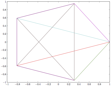
Run pdflatex myfile in the terminal. If everything is correctly set up, you will obtain mydoc.pdf. This is what the image part of the document should look like (click any image to download underlying pdf):

The alignment might be strange, but we can notice that the font of the tick marks is that of the LaTex document, rather than that used in Matlab. Now that we have basic functionality, let's first work on getting the picture pretty, then on how to use it in the LaTex document.

Pretty Plots

This section contains one example of how to make a pretty plot. Much more can be learnt by reading the PGF/TikZ manual (which is very well written but several 100 pages long.)

Automating Generation and Sizing

First, create an m-file with name of your choice containing the following:

plot(dftmtx(5)); % same as previous example
box off

% save the picture programatically
matlab2tikz('myfig2.tikz','height','\pgfigheight','width','\pgfigwidth')

When run, the above m-file will generate the file myfig2.tikz. Note that you can invoke matlab2tikz multiple times from the same m-file. It will always act on the active figure. If you open myfig2.tikz in a text editor and compare it to myfig.tikz, you will see that the width and height specifications have changed from fixed numbers into \pgfigwidth and \pgfigheight, respectively. These can be set in your LaTex document, to change the dimensions of the important graphic. Modify mydoc.tex:

\documentclass{pm}
\usepackage{tikz,pgfplots}
\newlength{\pgfigheight}
\newlength{\pgfigwidth}
\begin{document}
\setlength{\pgfigheight}{5cm}
\setlength{\pgfigwidth}{.8\linewidth}
\input{myfig2.tikz}
\end{document}

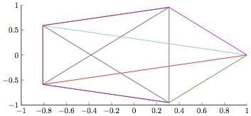
Try it out. Alignment is still not pretty, but the dimensions of the figure are now easy to set. (You can change \pgwidth and \pgheight throughout the document, to import graphics of different dimensions.) This is what the image part of the document should look like:

Axis and Labels

Now create a file called e.g. tikzdefs.tex:

\usetikzlibrary{narrow}
\tikzset{>=narrow}

\pgfplotsset{compat=1.3,
every axis/.append style={thin},
tick style={black,thin},                                                                  
major tick length={3pt},
tick align={inside},
/pgf/number format/1000 sep={},
every axis x line/.style={bottom},
every axis y line/.style={left},
every outer x axis line/.append style={-narrow},
every outer y axis line/.append style={-narrow},
every outer z axis line/.append style={-narrow},
every axis x label/.append style={at={(1,0)},anchor=north east,yshift=-2pt},
every axis y label/.append style={at={(0,1)}, anchor=north east,rotate=-90,xshift=-2pt},
every 3d description/.append style={
every axis x label/.style={at={(ticklabel cs:1.0)},anchor=north east},
every axis y label/.style={at={(ticklabel cs:1.0)},anchor=north west},
every axis z label/.style={at={(ticklabel cs:1.0)},anchor=south east},
every outer y axis line/.append style={-}
}
}

This file defines the axis style (and some other properties). To learn more, search for the key words in the PGF/TikZ manual and change them according to your taste. If you make useful changes, feel free to add them to this page! The string -narrow specifies an arrow style developed at the department, defined in tikzlibrarynarrow.code.tex.

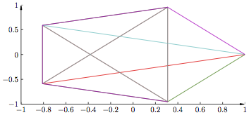
In mydoc.tex, include the line \input{tikzdefs} right after begin{document}, compile and have a look:

There are annoying tick marks at the arrow ends and we do not have any labels. Go back to the m-file and change it into:

plot(dftmtx(5)); % same as previous example
box off

% configure ticks and tick labels
set(gca,'XTick',-1:.2:.8)
set(gca,'YTick',[-1 0 .5])
set(gca,'YTickLabel',{'A','B','Q'})

% labels
xlabel('$t$')
ylabel('$\sqrt{\pi}$')

% save the picture programatically
matlab2tikz('myfig2.tikz','height','\pgfigheight','width','\pgfigwidth','parseStrings',false)

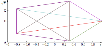
The changes allow for manual configuration of tick marks and labels. The 'parseString',false argument tells matlab2tikz to pass strings (e.g. xlabel), unmodified to the output file.

This is what the graphics part of the resulting pdf looks like:

Deviating from Style Template

A situation might occur, where you want a specific graphic to deviate from the style defined in tikzdefs.tex. This can be done in matlab2tikz by adding the extraAxisOptions argument. An example is provided below:

plot(dftmtx(5)); % same as previous example
box off

% configure ticks and tick labels
set(gca,'XTick',-1:.2:.8)
set(gca,'YTick',[-1 0 .5])
set(gca,'YTickLabel',{'A','B','Q'})

% labels
xlabel('$t$')
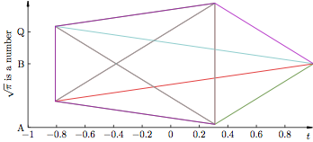
ylabel('$\sqrt{\pi}$ is a number')

% save the picture programatically
matlab2tikz('myfig2.tikz','height','\pgfigheight','width','\pgfigwidth','parseStrings',false,...
    'extraAxisOptions',...
    'y label style={at={(ticklabel cs:.5)},rotate=90,anchor=south,yshift=-2mm}')

Run it, and recompile the LaTex document to see the results (the y axis label is changed). Also open myfig2.tikz in a text editor to see what extraAxisOptions does. The resulting graphics:

Of course, you can achieve these changes by editing the .tikz-files as well, but this would add the need of manual intervention when re-compiling your document from scratch.

Make it fast and less memory dependent

Faster and requiring less memory

Sometimes it takes ages for pdflatex to compile TikZ graphics, and occasionally pdflatex runs out of memory. It is possible to increase the memory allowance (and wait longer), but there are better alternatives.

Since the graphics are all vector based, consider removing unnecessary data points. For instance x=0:1e-7:1;y=sin(x),plot(x,y) is overkill. It is here enough to use e.g. x=0:1e-2:1. An alternative to doing this prior to plotting is to add 'minimumPointsDistance', 0.025e-3 to the argument list of matlab2tikz. The number argument can be changed to provide the sought file size-resolution tradeoff.

The official version of matlab2tikz downsamples the image uniformly to achieve minimumPointDistance. There is a non-supported version of matlab2tikz, which uses a more clever downsampling algorithm, which preserves higher resolution in parts of the graphic where they are needed. On the department computers, this version is available as matlab2tikz2. The minimumPointDistance argument still dictates the file size-resolution tradeoff, but its meaning is not verbatim.

Decrease recompilation time

If you have a document with many graphics, it can take quite a while for pdflatex to compile it, even if the production of each individual graphic is optimized, as described above. A good thing is that TikZ supports the cashing of precompiled pdf files holding the graphics. We will now go through how to set this up.

In this example we will assume you have a file mydoc.tex:

\documentclass{pm}
\usepackage{tikz,pgfplots}
\usetikzlibrary{external}\tikzexternalize
\tikzsetexternalprefix{./}
\newlength{\pgfigheight}
\newlength{\pgfigwidth}
\begin{document}
\input{tikzdefs}
\setlength{\pgfigheight}{5cm}
\setlength{\pgfigwidth}{.8\linewidth}
\input{myfig2.tikz}
\end{document}

and that myfig2.tikz is the file created in the above example. The tikzexternalize library is what does the job for us. In this example tikzexternalprefix is useless. However, in case you want the (pdf) cache files sorted in e.g. a directory figs, you will want to use \tikzsetexternalprefix{./figs/}.

To compile, pdflatex needs to have shell escapes enabled. This is done by invoking it as pdflatex -shell-escape mydoc. (If you do this often, it might be useful to add the following line to your .bash_profile file found in your home directory. If you don't have one already, create it by typing cd;touch .bash_profile in the terminal. Then edit it and add the line:

alias pdflatex='pdflatex -shell-escape'

Once you compile mydoc.tex, some files with names starting with mydof-figure0 are created. Among these are mydoc-figure0.pdf containing your figure (open it to have a look). Upon consecutive compilations, pdflatex will first check if mydoc-figure0.pdf exists. Only if it does not, will the underlying TikZ file be processed. Therefore, if you make changes to the m-file generating the Tikz file or the Tikz file itself, don't forget to delete mydoc-figure0.pdf before recompiling your document.

It might be a bit hard to find the appropriate pdf file to delete if you have many graphics. A good idea is therefore to add the following section to tikzdefs.tex:

\newcommand{\tikzin}[1]{
\centering
\tikzsetnextfilename{#1.precompiled}
\input{#1}
}

and replace \input{myfig2.tikz} in mydoc.tex by \tikzin{myfig2.tikz}. This ensures that the pre-compiled pdf will hold the same base name as the underlying TikZ file.

Including Graphics

Now that we have the files myfig2.tikz and tikzdefs.tex, let's change mydoc.tex into something a bit closer to a real-world example:

\documentclass{pm}
\usepackage{tikz,pgfplots}
\usetikzlibrary{external}\tikzexternalize
\tikzsetexternalprefix{./}
\newlength{\pgfigheight}
\newlength{\pgfigwidth}
\begin{document}
\input{tikzdefs}
\setlength{\pgfigheight}{5cm}
\setlength{\pgfigwidth}{.8\linewidth}
Something is shown in Figure~\ref{fig:picture}.                         
\begin{figure}
\tikzin{myfig2.tikz}
\caption{This is a picture.\label{fig:picture}}
\end{figure}
\end{document}

The resulting file should look like this:

Hint: If you have several figures that you want to vertically align at their axis, add 'extraTikzpictureSettings','trim axis left,trim axis right' to the argument list of matlab2tikz (in the m-file). This trims the bounding box of the resulting pdf to the axis. Then you can align the figures (left or right, but not centered) under each other to obtain alignment at their axis.